Hooke's Law: Nonlinear Generalization and Applications
Part I: The generalized law
Prof. Dr. Hans Schneeberger
Institute of Statistics, University of Erlangen-Nürnberg, Germany
2020, 08th of June
Keywords: Linear growing process; superposed exponential dying process; mathematics of cracks.
Introduction
Hooke’s Law (Hooke 1635-1703) is well-known as the linear relation of stress σ and strain ε with elastic materials:
σ=aε(1)
But it is also known for a long time, that this linearity is (nearly) right only for smaller values of ε.
As I use data of different authors with different units of measurement and also for simplification I will use terms x for strain ε and y for stress σ. And as it is usual in mathematical statistics, i will distinguish data-values (e.g. y) and hypothetical values (e.g. ŷ). Hooke’s Law then is
ŷ=ax(2)
My generalized hypothesis is:
ŷ=axe-bx(3)
that means, that a linear growing process ax (a>0) – Hooke’s process - is superposed by an exponential declining or dying process e(-bx) (b>0).
Hooke’s process (2) is a first approximation of process (3). For writing e(-bx) as Taylor-series, we have
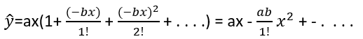
and so ŷ∼ax for small values of x.
In this paper I will show with three characteristic experiments of centrically pressed prisms and cubes the corresponcence of data and hypothesis (3).
A following part II will give the generalization for noncentrically pressed prisms and cubes and resulting laws of the bending pressure zone.
And a part III gives the distribution of the stress in the cross-section of a beam in dependence on the strength of the material and of the loading.
Experiments and Results
(I) Experiment of the University of Technology Munich [4]
In figure 1a the stress-strain lines of centrically pressed prisms in short-time pressing are given (in reduced size).
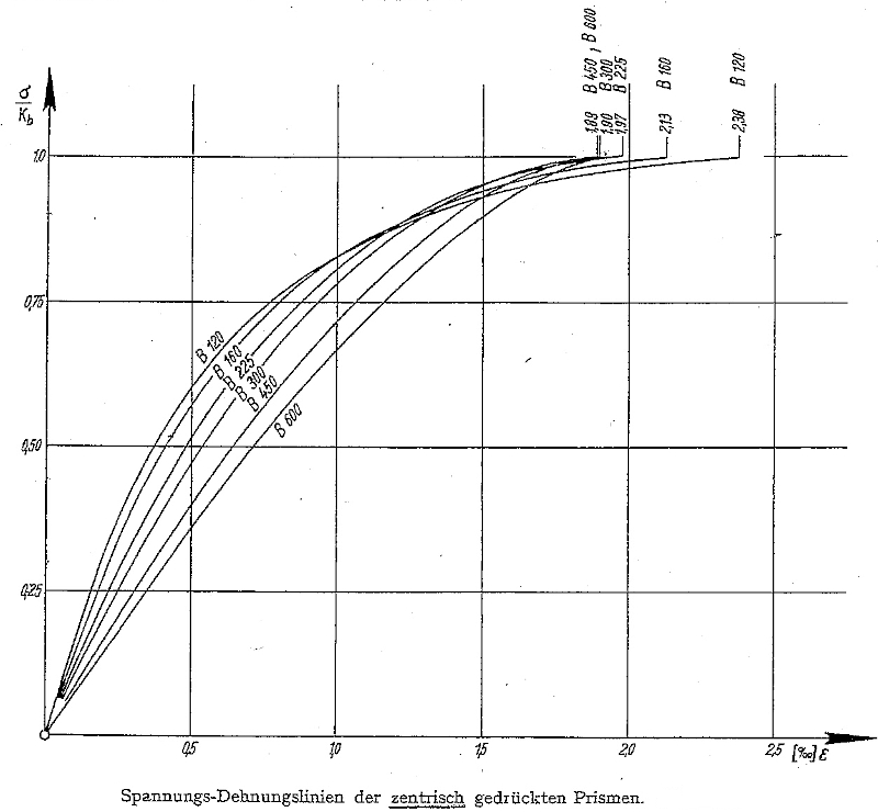
Fig. 1a: Experimental stress-strain curves
To make use of this data-basis to test my hypothesis (3), I chose as data-points n=7 (x,y)-values from each of the four curves B160, B300, B450 and B600 - see table 1.
| x | .2 | .4 | .6 | .8 | 1 | 1.2 | 1.4 | |
|---|---|---|---|---|---|---|---|---|
| B160 | y | .28 | .50 | .64 | .75 | .83 | .88 | .92 |
| B300 | y | .21 | .39 | .55 | .68 | .785 | .865 | .93 |
| B450 | y | .16 | .325 | .47 | .60 | .715 | .815 | .90 |
| B600 | y | .145 | .29 | .43 | .555 | .67 | .765 | .86 |
x is strain ε (in promille); y is stress σ/strenth Kb of prism;
B160 means strength 160(kg/cm2) of concrete; similar B300etc.
The mathematical problem is the optimal approximation of experiment and hypothesis. This is done by the method of least sqares of Gauss
Q(a,b)=∑(yi - ŷl)2
(summing from 1 to n). The optimal parameters a and b are found with the iterative non-linear simplex-method of Nelder and Mead [1]. The results are:
B160 ŷ=1.563 × e-0.6263x
B300 ŷ=1.159 × e-0.3953x
(4)
B450 ŷ=0.9009 × e-0.2372x
B600 ŷ=0.797 × e-0.1835x
See figure 1b.
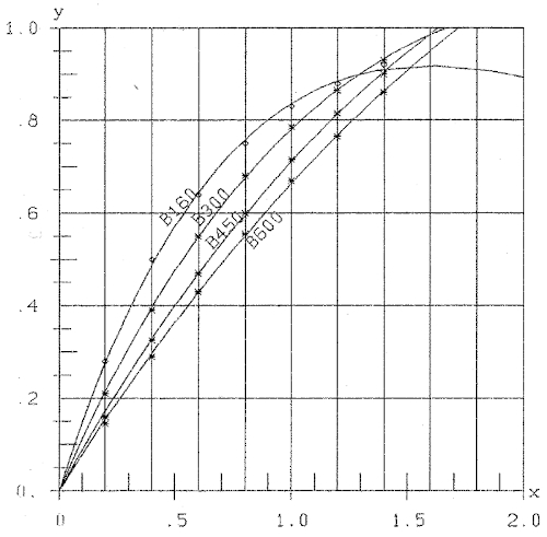
Fig. 1b: Stress-strain curves ŷ=a×e(-bx)
The corresponding straight lines of Hooke are ŷ=ax, i.e. ŷ=1.563x for B160 etc. That are the tangents to the curves (4) in the point (x,y)=(0,0).
(II) Experiment of the University of London: City and Guilds College [2]
Prentis concludes in his paper ([2], p.75), that „the basic differences between the various plastic theories for reinforced beams result mainly from differences of opinion as to the form of the curve, and it is hoped that applications of the above analysis will help to resolve the problem“.
Figure 2a gives a copy of Prentis' result-curve on a scale of 1:1. To make the analogous calculation as in experiment (I), I chose n=8 data-points of this curve, which are given in table 2.
| x | .5 | 1 | 1.5 | 2 | 2.5 | 3 | 3.5 | 3.83 |
|---|---|---|---|---|---|---|---|---|
| y | 1.659 | 2.723 | 3.404 | 3.744 | 4.000 | 4.084 | 4.042 | 3.914 |
x=1 corresponds to strain ε=0.001(inches/inch)
y=1 corresponds to stress σ=1000(lb/sq.in.)
The resulting optimal stress-strain curve is:
ŷ=3.789 ×e-0.3422x(5)
which is plotted in figure 2b. Hooke’s line straight line is ŷ=3.789x.
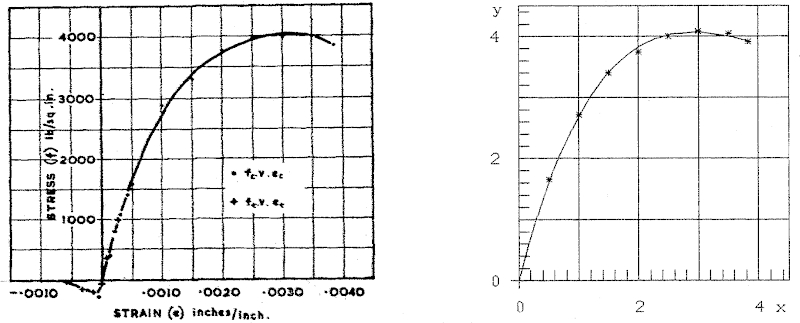
Fig.2a: Experimental stress-strain curve Fig.2b: Stress-strain curve ŷ=a×e(-bx)
(III) Experiment of the University of Technology Munich with dε/dt=const. and with cracks [3]
In figure 3a (in reduced size) the result of the experiment is given: Cube strength W=244 kp/cm2, dε/dt=0.1%/1.875min.
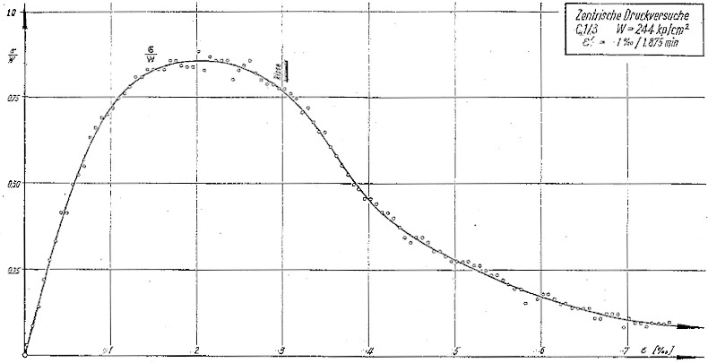
Fig. 3a: Experimental stress-strain curve
For computation n=27 data-points (x,y) are read from the curve in figure 3a and are given in table 3.
| x | .2 | .4 | .6 | .8 | 1 | 1.2 | 1.4 | 1.6 | 1.8 | 2 | 2.2 | 2.4 | 2.6 | 2.8 | 3 |
|---|---|---|---|---|---|---|---|---|---|---|---|---|---|---|---|
| y | .212 | .382 | .523 | .630 | .717 | .773 | .821 | .845 | .853 | .856 | .857 | .845 | .821 | .798 | .7768 |
| x | 3.2 | 3.4 | 3.6 | 3.8 | 4 | 4.5 | 5 | 5.5 | 6 | 6.5 | 7 | 7.5 | - | - | - |
| y | .702 | .649 | .583 | .508 | .456 | .345 | .274 | .214 | .167 | .131 | .104 | .088 | - | - | - |
x is strain ε (in promille); y is stress σ/strength W of cube
At first the parameters a and b of formula (3) were estimated with all 27 data; the result
ŷ=1.383 ×e-0.5996x
is given in figure 3b
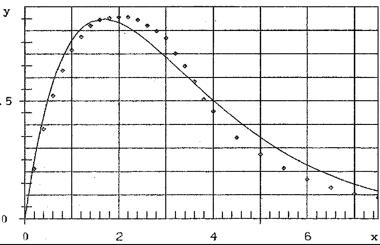
Fig. 3b: Stress-strain curve ŷ=a×e(-bx); parameter-estimation with all data
Surely one can not claim, that the correspondence of data-points and hypothetical curve is good.
So I supected, that the reason is the crack at x0∼3 (see figure 3a) and computed the parameters a and b with formula (3) only with the 15 data points (x,y)=(0.2,0.212), . . . , (3,0.768) –up to the crack. The result is
(A) ŷ=1.188 ×e-0.5093x(6)
and is given as curve A in figure 3c.
We have a very good correspondence of data and hypothesis up to the point of crack. Then the declining of the data-values y is stronger than that of the hypothetical curve (6) or: the growing of the growing part ax of formula (3), that is y=ax, is too strong. So I made the simplest alternative hypothesis: With the crack the growing part of formula (3) „cracks“ too: ax → ax0=const. for x≥x0. So for x≥x0 I made the hypothesis
ŷ=ce-bx, c=ax0
and computed the parameters c and b with the n=13 data-points (x,y)=(3.0,0 .768) . . , (7.5,0.088). The result is
(B) ŷ=3.640e-0.5148x(7)
curve B in figure 3c. Correspondence of data and hypothesis is again very good, I think.
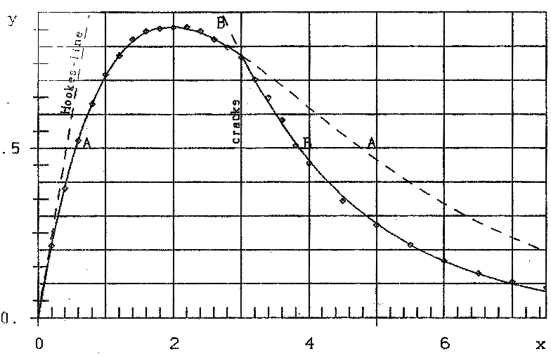
Fig.3c Stress-strain curves A: before the crack, B: after the crack
Comparison of formulae (A) and (B) show:
- the exponents b are (practically) the same: b=0.51
- ax0=1.188*3=3.564 from (A) is (practically) c=1.213*3=3.640 (from (B))
(Consider that x0 is not exaxtly fixed and that the data-points are result of one experiment).
So the final formula is (see figure 3d)
ŷ=1.20xe-0.51x for x≤x0(8a)
and
ŷ=1.20x0e-0.51x for x≥x0(8b)
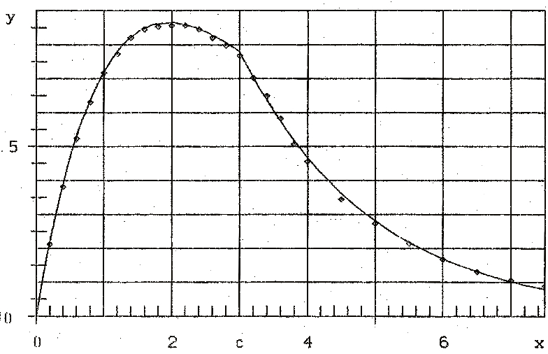
Fig. 3d: Combined stress-strain curve
i.e. up to the cracking point x0 Hooke’s linear growing process ax=1.20x is superposed by an exponential dying process with parameter 0.51 according to formula (8a). In the cracking point Hooke’s growing process „cracks down“ to a constant ax0; a simple exponential dying process (8b) is left – with the same parameter 0.51 as before.
References
[1] Nelder, J.R. and Mead, R. (1965). A Simplex Method for function minimization. The Computer Journal, 7, 303-313.
[2] Prentis, J.M. (1951). The distribution of stress in reinforced and prestressed concrete beams when tested to destruction by a pure bending moment. Magazine of Concrete Research, no.5, Cement and Concrete Ass., London.
[3] Rasch, Ch. (1962). Spannungs-Dehnungs Linien des Betons und Spannungsverteilung in der Biegedruckzone bei konstanter Dehngeschwindigkeit. Deutscher Ausschuß für Stahlbeton, Heft 154.
[4] Rüsch, H. (1955). Versuche zur Festigkeit der Biegedruckzone. Deutscher Ausschuß für Stahlbeton, Heft 120.
Download this paper as PDF
Download this Paper in PDF format:
Hooke's Law: Nonlinear Generalization and Applications. Part I: The generalized law [PDF, 561 kB]