Hooke's Law: Nonlinear Generalization and Applications
Part 3: Distribution of Stress in Prisms and Beams
Prof. Dr. Hans Schneeberger
Institute of Statistics, University of Erlangen-Nürnberg, Germany
2021, 26th of October
Introduction
As stated in [5], part II, the distribution of stress σ in the bending pressure zone of a beam is identical with the distribution of stress in a non-centric loaded prism in such a manner, that the strain ε2, remote to the loading, is zero (see figure 1).
In a huge number of experiments with the variables
ε1 (0/00 = ε0 (in contrast to ε2=0)
x=1-β0, the center of loading; NB! The width of the prism d=150cm (see [5], part II, figure 2) is standardized to 1: 0 ≤ x = ≤ 1 = d/150,
 , the (relative) loading; 𝐾b(kg/cm2) is the utmost strength of the prism with centric loading - Generally: Index 0 means „experiment with ε2=0“,
in [2] the experimental results are given in dependence on strength of cube W=W20 (kg/cm2; cube length 20 cm) and  (B for break). See also tables 1, 2, 3 and figures 4, 5 and 6 of [5], part II.
With these experimental data 3 hypothesis were postulated in II (hypothetical values are signed as  in contrast to experimental values
  – as it is usus in statistics).
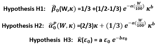
The good coincidence of experiments and hypotheses can be seen in the tables and figures of [5], part II.
Distribution of stress σ in an eccentric pressed prism (with ε2=0)
The (relative) stress y(x)=σ(x)/Κb is
Hypothesis 4: y(x)=Axe-Bx

Fig. 1: Sketch of an eccentrically pressed prism with center of pressure x=1-β0 so, that ε2=0
see figure 1. That means: The stress-function σ(x) for eccentric pressed prisms is of the same mathematical form as for centric pressed prisms, as Κb, as well as W, is a constant for a fixed experiment.
The two parameters A and B are estimated by minimizing according to the method of least squares of Gauss

together by minimizing the objective function D=D1+D2.
The values of  and
and  are given in [5], part II, tables 2 and 1 for a series of values of W and of κ
For example for W=300 and κ=0,9 we have 0.653 and 0.374.
The minimum of D is found by the iterative nonlinear Simplex-method of Nelder and Mead [1]. The resulting optimal parameters A and B of hypothesis H4 are registerd together with figure 2 for W=80, figure 3 for W=160, figure 4 for W=300, figure 5 for W=450 and figure 6 for W= 600 (kg/cm2). To every value of W seven values of κ = 0.3, 0.4, … 0.9 were chosen for stress-lines. For κ>0.9 and W< 80 I do not put my hand in the fire with my formulae. This may already be seen in figure 5b of [5], part II for κ=0.9 and small values of W.

Fig. 2: W=80 kg/cm². stress-lines y=Axe-Bx and strain ε0 according to H3 ([5], part II):  =aε0e-bε0
| κ | 0.3 | 0.4 | 0.5 | 0.6 | 0.7 | 0.8 | 0.9 |
|---|---|---|---|---|---|---|---|
| A | 0.4082 | 0.5601 | 0.7577 | 1.0230 | 1.4540 | 2.1750 | 3.5630 |
| B | 0.0306 | 0.0663 | 0.1726 | 0.3295 | 0.5850 | 0.9321 | 1.4280 |

Fig. 3: W=160 kg/cm². stress-lines y=Axe-Bx and strain ε0 according to H3 ([5], part II): =aε0e-bε0
| κ | 0.3 | 0.4 | 0.5 | 0.6 | 0.7 | 0.8 | 0.9 |
|---|---|---|---|---|---|---|---|
| A | 0.4057 | 0.5551 | 0.7325 | 0.9661 | 1.3080 | 1.8530 | 2.7990 |
| B | 0.0199 | 0.0556 | 0.1284 | 0.2532 | 0.4463 | 0.7235 | 1.1050 |

Fig. 4: W=300 kg/cm². stress-lines y=Axe-Bx and strain ε0 according to H3 ([5], part II): =aε0e-bε0
| κ | 0.3 | 0.4 | 0.5 | 0.6 | 0.7 | 0.8 | 0.9 |
|---|---|---|---|---|---|---|---|
| A | 0.4035 | 0.5470 | 0.7070 | 0.8996 | 1.1530 | 1.5110 | 2.0590 |
| B | 0.0126 | 0.0358 | 0.0805 | 0.1586 | 0.2810 | 0.4581 | 0.7037 |

Fig. 5: W=450 kg/cm². stress-lines y=Axe-Bx and strain ε0 according to H3 ([5], part II): =aε0e-bε0
| κ | 0.3 | 0.4 | 0.5 | 0.6 | 0.7 | 0.8 | 0.9 |
|---|---|---|---|---|---|---|---|
| A | 0.4019 | 0.5415 | 0.6904 | 0.8587 | 1.0600 | 1.3170 | 1.6680 |
| B | 0.0071 | 0.0217 | 0.0485 | 0.0966 | 0.1708 | 0.2792 | 0.4309 |

Fig. 6: W=600 kg/cm². stress-lines y=Axe-Bx and strain ε0 according to H3 ([5], part II): =aε0e-bε0
| κ | 0.3 | 0.4 | 0.5 | 0.6 | 0.7 | 0.8 | 0.9 |
|---|---|---|---|---|---|---|---|
| A | 0.4014 | 0.5380 | 0.6813 | 0.8341 | 1.0080 | 1.2110 | 1.4650 |
| B | 0.0054 | 0.0125 | 0.0306 | 0.0573 | 0.1038 | 0.1691 | 0.2636 |
In the left part of the figures the disrtribution of stress y is given.
The strain ε is zero for x=0 according to the experiments. For x=1 strain ε=ε0 can be computed with formulae =aε0e-bε0 of [5], part II. This is shown in the right part of the figures. For example in the experiment with W=300 and some values of we get (see also figure 4):
|
.3 | .4 | .5 | .6 | .7 | .8 | .9 |
|---|---|---|---|---|---|---|---|
| ε0 | .39 | .55 | .72 | .92 | 1.16 | 1.45 | 1.86 |
Distribution of stress σ in the bending pressure zone of a beam
According to [5], part II the distribution of the stress in the bending pressure zone of a beam is identical with that of a corresponding eccentric pressed prism with ε2=0: The side of the prism with ε=0 (y-axis in figure 1) is equivalent with the neutral axis of the beam (see figure 7).

Fig. 7: Sketch of the bending pressure zone of a beam
In figures 8, ..., 12 the lower part give the stress-lines in the bending pressure zones of the beams. They simply are the mirror-images of the stress lines of the corresponding prisms, reflected at the mirror with y=x.
The curves =aε0e-bε0 in the upper part of the figures are the same as those of the corresponding prisms (in a somewhat modified scale).

Fig. 8: W=80 kg/cm². Strain ε0 and stress-lines 
In the bending pressure zone 0 ≤ x ≤ 1

Fig. 9: W=160 kg/cm². Strain ε0 and stress-lines
In the bending pressure zone 0 ≤ x ≤ 1

Fig. 10: W=300 kg/cm². Strain ε0 and stress-lines
In the bending pressure zone 0 ≤ x ≤ 1

Fig. 11: W=450 kg/cm². Strain ε0 and stress-lines
In the bending pressure zone 0 ≤ x ≤ 1

Fig. 12: W=600 kg/cm². Strain ε0 and stress-lines
In the bending pressure zone 0 ≤ x ≤ 1
Comment
The experiments, the results of which are used in this analysis, were directed by Rüsch [2] at the University of Technology Munich. The evaluation of the data was done under the direction of Scholz, who also made two hypotheses on the distribution of the stress in beams ([3] and [4]).
References
[1] Nelder, J.R. and Mead, R. (1965). A Simplex Method for function minimization. The Computer Journal, 7, 303-313.
[2] Rüsch H. (1955). Versuche zur Festigkeit der Biegedruckzone. Deutscher Ausschuß für Stahlbeton, Heft 120
[3] Scholz G.(1957). Über die wahrscheinlichste Spannungsverteilung in der Biegedruckzone von Stahlbetonbalken mit rechteckigem Querschnitt. Dissertation
[4] Scholz G. 1960). Festigkeit der Biegedruckzone, Heft 139. Deutscher Ausschuss für Stahlbeton, Heft 139
[5] Schneeberger H. (2020). Hooke's Law: Nonlinear Generalization and Applications.
Download this paper as PDF
Download this Paper in PDF format:
Hooke's Law: Nonlinear Generalization and Applications. Part 3: Distribution of Stress in Prisms and Beams [PDF, 722 kB]